Reinforcement Learning - MDP and RL

What is Reinforcement Learning?

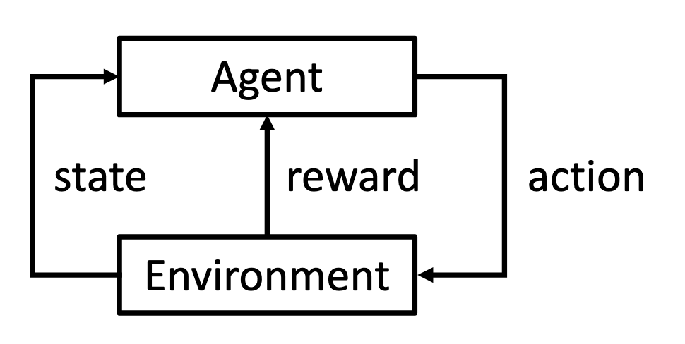
A typical Reinforcement Learning system consists of 5 components: an agent takes an action at each state in an environment and receives a reward if some criteria are met.

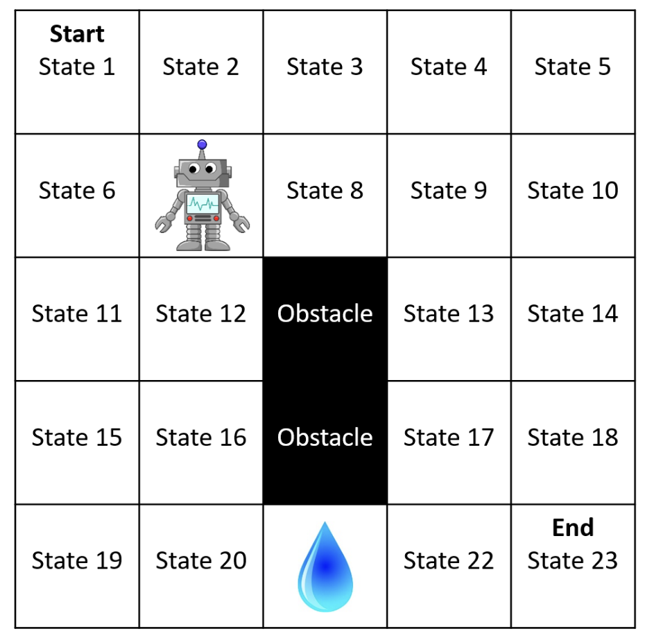
Example: Gridworld

State: Position of robot. The robot does not have a direction that it is facing.

Actions: Attemp_Up (AU), Attemp_Down (AD), Attemp_Left (AL), Attemp_Right (AR)

Environment Dynamics:

Rewards:

• The agent receives a reward of -10 for entering the state with the water and a record of +10 for entering the goal state.
• Entering any other state results in a reward of zero.
• Any actions that cause the agent stays in state 21 will count as “entering” the water state again and result in an additional reward of -10.
• Reward discount parameter \(\gamma = 0.9\).

Number of States: 24

• 23 normal states + 1 terminal absorbing state (\(s_\infty\))
  • Once in \(s_\infty\), the agent can never leave (episode ends).
  • \(s_\infty\) should not be thought as “goal” state.

---

Describe the Agent and Environment Mathematically

Math Definition for Environment

We can use Markov Decision Processes (MDPs) to formalize the environment of an RL problem. The unique terms are \(\mathcal{S}\) (the set of all possible states), \(\mathcal{A}\) (the set of all possible actions), \(p\) (transition function), \(d_R\) (reward distribution), \(R\) (reward function), \(d_0\) (initial state distribution), and \(\gamma\) (reward discount parameter). The common definition of the environment is

\[(\mathcal{S}, \mathcal{A}, p, R, \gamma)\]

Math Definition for Agent

We define the decision rule that the agent selects actions as a policy. Formally, a policy \(\pi\) is a function

\[\begin{aligned} &\pi : \mathcal{S} \times \mathcal{A} \rightarrow [0,1] \\ &\pi(s,a) := \text{Pr}(A_t=a | S_t=s) \end{aligned}\]

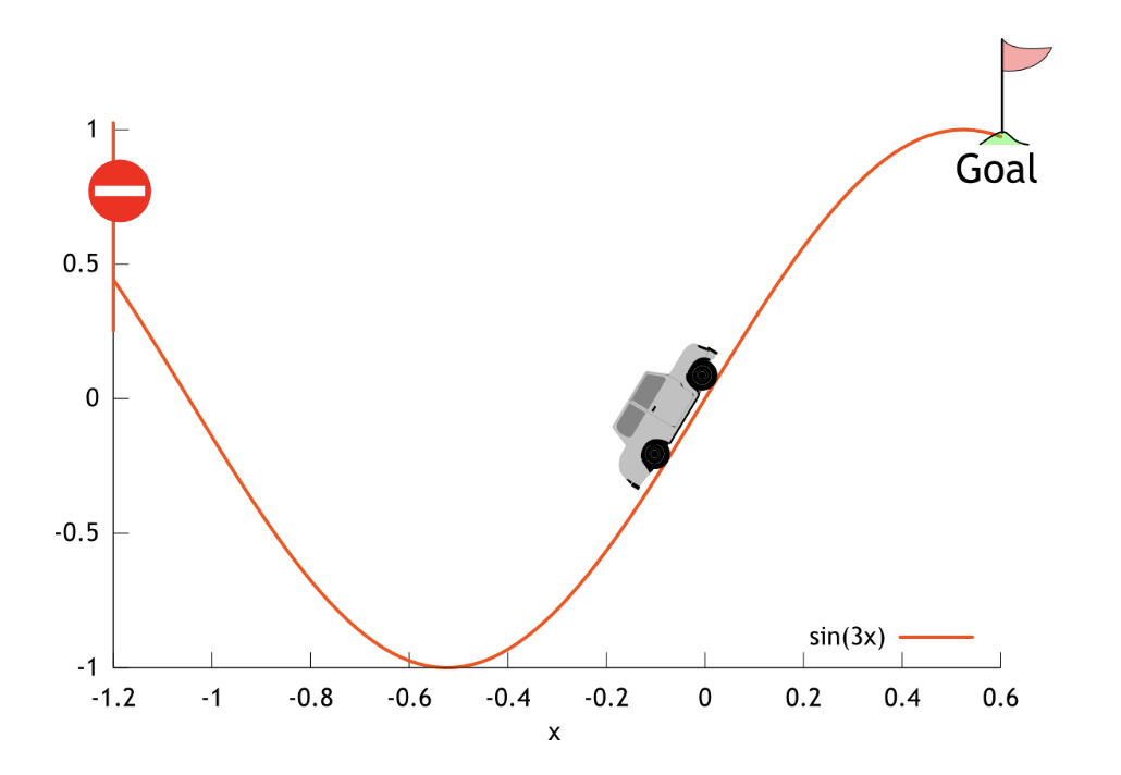
Example: Mountain Car

• State: \(s=(x,v)\), where \(x \in \mathbb{R}\) is the position of the car and \(v \in \mathbb{R}\) is the velocity.
• Actions: \(a \in \{\texttt{reverse}, \texttt{neutral}, \texttt{forward}\}\). These actions are mapped to numerical values as \(a \in \{-1, 0 ,1\}\).
• Dynamics: The dynamics are deterministic—taking action \(a\) in state \(s\) always produces the same state, \(s^\prime\). Thus, \(p(s,a,s^\prime) \in \{0, 1\}\). The dynamics are characterized by:

\[\begin{aligned} v_{t+1} &= v_t + 0.001 a_t - 0.0025 \cos(3x_t) \\ x_{t+1} &= x_t + v_{t+1} \end{aligned}\]

After the next state, \(s^\prime = [x_{t+1}, v_{t+1}]\) has been computed,

• the value of \(x_{t+1}\) is clipped so that it stays in the closed interval \([-1.2, 0.5]\).
• the value of \(v_{t+1}\) is clipped so that it stays in the closed interval \([-0.7, 0.7]\).

• if \(x_{t+1}\) reaches the left or right bound (\(x_{t+1} = -1.2\) or \(x_{t+1} = 0.5\)), then the car’s velocity is reset to zero (\(v_{t+1} = 0\)).

• Initial State: \(S_0 = (X_0, 0)\), where \(X_0\) is an initial position drawn uniformly at random from the interval \([-0.6, -0.4]\).
• Terminal States: If \(x_t = 0.5\), then the state is terminal (it always transitions to \(s_\infty\)).
• Rewards: \(R_t = -1\) always, except when transitioning to \(s_\infty\) (from \(s_\infty\) or from a terminal state), in which case \(R_t = 0\).
• Discount: \(\gamma = 1.0\).

---

Additional Terminology, Notation, and Assumptions

• A history, \(H_t\), is a recording of what has happened up to time \(t\) in an episode:

\[H_t := (S_0, A_0, R_0, S_1, A_1, R_1, \ldots, S_t, A_t, R_t)\]

• A trajectory is the history of an entire episode: \(H_\infty\)
• The return or discounted return of a trajectory is the discounted sum of rewards \(G := \sum_{t = 0}^{\infty} \gamma^t R_t\)
• The expected return or expected discounted return can be written as \(J(\pi) := \mathbf{E}[G\vert\pi]\)
• The return from time \(t\) or discounted return from time \(t\), \(G_t\), is the discounted sum of rewards starting from time \(t\)

\[G_t := \sum_{k=1}^{\infty} \gamma^k R_{t+k}\]

• The horizon, \(L\), of an MDP is the smallest integer such that \(\forall t \geq L, \text{Pr}(S_t = s_\infty) = 1\)
  • if \(L < \infty\) for all policies, then we say that the MDP is finite horizon
  • if \(L = \infty\) then the domain may be indefinite horizon (the agent will always enter \(s_\infty\)) or infinite horizon (the agent may never enter \(s_\infty\))

---

Markov Property

If a model (environment, reward …) holds the Markov assumption, we say it has the Markov property, or say the model is Markovian.

---

Why use MDP in RL?

MDP is not only powerful enough to model the interaction between a learning agent and its environment, it also brings some critical guarantees that make our “reinforcement learning” actually work.

For now, let’s skip the derivation and jump straight to the conclusions.

Later when we introduce the Bellman equation and the Bellman optimality equation, we will further establish that:

1. if a policy \(\pi\) achieves a state where its expected future rewards cannot be improved further by any other action or decision at each step (Bellman optimality equation), then it is an optimal policy.
2. if there are only a finite number of possible states and actions, rewards are bounded, and future rewards are discounted (with a discount factor \(\gamma < 1\)), then there exists a policy \(\pi\) that satisfies the Bellman optimality equation.

Furthermore, we can perform policy/value iteration (will be covered later) using the Bellman and Bellman optimality equation. As a result, we can not only get better policies iteration after iteration, but also, under some constraints, prove that the final policy will converge to the optimal policy.