Reinforcement Learning — Value Functions

Last time, we covered how MDPs are integrated into Reinforcement Learning. In this chapter, we will see how we can evaluate an RL agent mathematically based on the definitions of MDPs.

State-Value Function

The State-Value function $v^\pi(s)$ calculates the expected discounted return if the agent starts in state $s$ and follows policy $\pi$. Informally, it tells us how “good” it is for the agent to be in state $s$ when using policy $\pi$. We call $v^\pi(s)$ the value of state $s$.

\[\begin{aligned} v^\pi(s) &:= \mathbf{E}\ \Bigg[\underbrace{\sum_{k=0}^{\infty}\gamma^k R_{t+k}}_{G_t} \bigg| S_t=s, \pi\ \Bigg] \\ &:= \mathbf{E}[G_t|S_t=s, \pi] \\ &:= \mathbf{E}\ \Bigg[\sum_{t=0}^{\infty}\gamma^k R_{t} \bigg| S_0=s, \pi\ \Bigg] \end{aligned}\]

Recalling the $G_t$ notation (discounted return from time $t$) we covered last time, we can see that this is an equivalent definition.

A Simple MDP Example

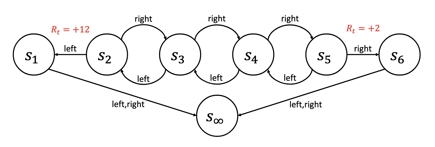
In the MDP above, the agent can choose between two actions: Left or Right. In states $s_1$ and $s_6$, any action will cause a transition to the terminal state $s_\infty$. The agent only gets a reward when transitioning from $s_2 \to s_1$ or $s_5 \to s_6$. For simplicity, we will use $\gamma = 0.5$.

Let’s test two policies for this MDP. One policy, $\pi_1$, will always select Left action; another policy, $\pi_2$, will always select the Right action.

Policy 1 ($\pi_1$): Select Left Action Always

$v^{\pi_1}(s_1) = 0$ (goes to the terminal state always)
$v^{\pi_1}(s_2) = 12\gamma^0 = 12$.
$v^{\pi_1}(s_3) = 0\gamma^0 + 12\gamma^1 = 6$.
$v^{\pi_1}(s_4) = 0\gamma^0 + 0\gamma^1 + 12\gamma^2 = 3$.
$v^{\pi_1}(s_5) = 0\gamma^0 + 0\gamma^1 + 0\gamma^2 + 12\gamma^3 = 1.5$.
$v^{\pi_1}(s_6) = 0$.

Policy 2 ($\pi_2$): Select Right Action Always

$v^{\pi_2}(s_1) = 0$.
$v^{\pi_2}(s_2) = 0\gamma^0 + 0\gamma^1 + 0\gamma^2 + 2\gamma^3 = 0.25$.
$v^{\pi_2}(s_3) = 0\gamma^0 + 0\gamma^1 + 2\gamma^2 = 0.5$.
$v^{\pi_2}(s_4) = 0\gamma^0 + 2\gamma^1 = 1$.
$v^{\pi_2}(s_5) = 2\gamma^0 = 2$.
$v^{\pi_2}(s_6) = 0$.

Action-Value Function

The Action-Value Function $q^\pi(s,a)$, or Q-function, evaluates the expected discounted return if the agent takes action $a$ in state $s$ and follows policy $\pi$ thereafter.

\[\begin{aligned} q^\pi(s,a) &:= \mathbf{E}\ \Bigg[\sum_{k=0}^{\infty}\gamma^k R_{t+k} \bigg| S_t=s, A_t = a, \pi\ \Bigg] \\ &:= \mathbf{E}[G_t|S_t=s, A_t=a, \pi] \\ &:= \mathbf{E}\ \Bigg[\sum_{t=0}^{\infty}\gamma^k R_{t} \bigg| S_0=s, A_0=a, \pi\ \Bigg] \end{aligned}\]

A Simple MDP Example, Again

Policy 1 ($\pi_1$): Select Left Action Always

$q^{\pi_1}(s_1, L) = 0$.
$q^{\pi_1}(s_1, R) = 0$.
$q^{\pi_1}(s_2, L) = 12\gamma^0 =12$.
$q^{\pi_1}(s_2, R) = 0\gamma^0 + 0\gamma^1 + 12\gamma^2 = 3$.
$q^{\pi_1}(s_3, L) = 0\gamma^0 + 12\gamma^1 = 6$.
$q^{\pi_1}(s_3, R) = 0\gamma^0 + 0\gamma^1 + 0\gamma^2 + 12\gamma^3 = 1.5$.
$q^{\pi_1}(s_4, L) = 0\gamma^0 + 0\gamma^1 + 12\gamma^2 = 3$.
$q^{\pi_1}(s_4, R) = 0\gamma^0 + 0\gamma^1 + 0\gamma^2 + 0\gamma^3 + 12\gamma^4 = 0.75$.
$q^{\pi_1}(s_5, L) = 0\gamma^0 + 0\gamma^1 + 0\gamma^2 + 12\gamma^3 = 1.5$.
$q^{\pi_1}(s_5, R) = 2\gamma^0 = 2$.
$q^{\pi_1}(s_6, L) = 0$.
$q^{\pi_1}(s_6, R) = 0$.

Policy 2 ($\pi_2$): Select Right Action Always

$q^{\pi_2}(s_1, L) = 0$.
$q^{\pi_2}(s_1, R) = 0$.
$q^{\pi_2}(s_2, L) = 12\gamma^0 =12$.
$q^{\pi_2}(s_2, R) = 0\gamma^0 + 0\gamma^1 + 0\gamma^2 + 2\gamma^3 = 0.25$.
$q^{\pi_2}(s_3, L) = 0\gamma^0 + 0\gamma^1 + 0\gamma^2 + 0\gamma^3 + 2\gamma^4 = 0.125$.
$q^{\pi_2}(s_3, R) = 0\gamma^0 + 0\gamma^1 + 2\gamma^2 = 0.5$.
$q^{\pi_2}(s_4, L) = 0\gamma^0 + 0\gamma^1 + 0\gamma^2 + 2\gamma^3 = 0.25$.
$q^{\pi_2}(s_4, R) = 0\gamma^0 + 2\gamma^1 = 1$.
$q^{\pi_2}(s_5, L) = 0\gamma^0 + 0\gamma^1 + 2\gamma^2 = 0.5$.
$q^{\pi_2}(s_5, R) = 2\gamma^0 = 2$.
$q^{\pi_2}(s_6, L) = 0$.
$q^{\pi_2}(s_6, R) = 0$.

The Bellman Equation for $v^\pi$

The Bellman Equation for $v^\pi$ is a recursive expression for the state-value function. To derive the Bellman equation, we first isolate the immediate reward from the state-value function:

\[\begin{aligned} v^\pi(s) &:= \textbf{E}\left[\sum_{k=0}^{\infty}\gamma^k R_{t+k} \bigg\vert S_t=s, \pi\right] \\ &= \textbf{E}\left[R_t + \sum_{k=1}^{\infty}\gamma^k R_{t+k} \bigg\vert S_t=s, \pi\right] \\ &= R_t + \textbf{E}\left[\gamma\sum_{k=1}^{\infty}\gamma^{k-1} R_{t+k} \bigg\vert S_t=s, \pi\right] \end{aligned}\]

We can perform a simple transformation by modifying the indexing of the sum to start at zero instead of one, which changes all uses of $k$ within the sum to $k+1$:

\[\begin{aligned} \textbf{E}\left[\gamma\sum_{k=1}^{\infty}\gamma^{k-1} R_{t+k} \bigg\vert S_t=s, \pi\right] = \textbf{E}\left[\gamma\sum_{k=0}^\infty \gamma^k R_{t+k+1} \bigg\vert S_t=s, \pi\right] \end{aligned}\]

Recalling the law of total probability, $\textbf{E}[X] = \textbf{E}[\textbf{E}[X\vert Y]]$, if we use the first action $A_t=a$ and the first next state $S_{t+1}=s^\prime$ as intermediate conditioning variables, we can rewrite the expected reward after the first action term as:

\[\begin{aligned} &\textbf{E}\left[\gamma\sum_{k=0}^\infty \gamma^k R_{t+k+1} \bigg\vert S_t=s, \pi\right] \\ = &\sum_{a\in\mathcal{A}}\pi(s,a)\sum_{s^\prime \in \mathcal{S}}p(s,a,s^\prime) \times \textbf{E}\left[\gamma\sum_{k=0}^\infty \gamma^k R_{t+k+1} \bigg\vert S_t=s, A_t=a, S_{t+1}=s^\prime, \pi\right] \end{aligned}\]

Furthermore, the Markov property tells us the future is independent of everything before $t+1$. Hence, for the expected next-step reward, we can safely remove $S_t$ and $A_t$ from the conditioning:

\[\begin{aligned} &\textbf{E}\left[\gamma\sum_{k=0}^\infty \gamma^k R_{t+k+1} \bigg\vert S_t=s, \pi\right] \\ = &\sum_{a\in\mathcal{A}}\pi(s,a)\sum_{s^\prime \in \mathcal{S}}p(s,a,s^\prime) \times \gamma\textbf{E}\left[\sum_{k=0}^\infty \gamma^k R_{t+k+1} \bigg\vert S_{t+1}=s^\prime, \pi\right] \end{aligned}\]

Recall the definition of the state-value function, the last term is exactly $v^\pi(s^\prime)$:

\[\begin{aligned} &\textbf{E}\left[\gamma\sum_{k=0}^\infty \gamma^k R_{t+k+1} \bigg\vert S_{t+1}=s^\prime, \pi\right] \\ = & \gamma\sum_{a\in\mathcal{A}}\pi(s,a)\sum_{s^\prime \in \mathcal{S}}p(s,a,s^\prime) v^\pi(s^\prime) \end{aligned}\]

Similarly, since for any fixed $s$ and $a$ the transition probability to the next state $s^\prime$ must be 1, we can multiply the immediate reward $R_t$ by “one”:

\[\begin{aligned} R_t = \sum_{a\in\mathcal{A}}\pi(s,a)R(s,a) = \sum_{a\in\mathcal{A}}\pi(s,a)\sum_{s^\prime \in \mathcal{S}}p(s,a,s^\prime)R(s,a) \end{aligned}\]

Now, we put everything together:

\[\begin{aligned} v^\pi(s) &= R_t + \textbf{E}\left[\gamma\sum_{k=0}^\infty \gamma^k R_{t+k+1} \bigg\vert S_t=s, \pi\right] \\ &= \sum_{a\in\mathcal{A}}\pi(s,a)\sum_{s^\prime \in \mathcal{S}}p(s,a,s^\prime)R(s,a) + \sum_{a\in\mathcal{A}}\pi(s,a)\sum_{s^\prime \in \mathcal{S}}p(s,a,s^\prime) \gamma v^\pi(s^\prime) \end{aligned}\]

Now, we can combine the common terms to get the final simplified form of the state-value function:

\[v^\pi(s) = \boxed{\sum_{a\in\mathcal{A}}\pi(s,a)\sum_{s^\prime \in \mathcal{S}}p(s,a,s^\prime)\big(R(s,a) +\gamma v^\pi(s^\prime)\big)}\]

Pros about Bellman Equation

We can view the Bellman equation as breaking the expected return that will occur into two parts:

the reward that we will obtain during the next time step (immediate reward)
the value of the next state that we end up in

\[v^\pi(s) = \textbf{E}\left[\underbrace{R(s,A_t)}_{\text{immediate reward}} + \gamma\underbrace{v^\pi(S_{t+1})}_{\text{value of next state}}\Bigg\vert S_t=s, \pi\right]\]

While the original definition of the value function must consider the entire sequence of states, the Bellman equation on the other hand, only needs to look forward one time step into the future.

the recurrent nature of the Bellman equation makes it more computationally helpful

The Bellman Equation for $q^\pi$

While the Bellman equation for $v^\pi$ is a recursive expression for $v^\pi$, the Bellman equation for $q^\pi$ is a recursive expression for the action-value function $q^\pi$.

\[\begin{aligned} q^\pi(s,a) &:= \mathbf{E}\Bigg[\sum_{k=0}^{\infty}\gamma^k R_{t+k} \bigg| S_t=s, A_t = a, \pi\Bigg] \\ &= R_t + \textbf{E}\left[\gamma\sum_{k=0}^\infty \gamma^k R_{t+k+1} \bigg\vert S_t=s, A_t = a, \pi\right] \\ &= R_t + \sum_{s^\prime \in \mathcal{S}}p(s,a,s^\prime)\sum_{a^\prime \in \mathcal{A}} \pi(s^\prime,a^\prime)\times\textbf{E}\left[\gamma\sum_{k=0}^\infty \gamma^k R_{t+k+1} \bigg\vert S_t=s, A_t = a, S_{t+1}=s^\prime, A_{t+1}=a^\prime, \pi\right] \\ &= R_t + \sum_{s^\prime \in \mathcal{S}}p(s,a,s^\prime)\sum_{a^\prime \in \mathcal{A}}\pi(s^\prime,a^\prime) \times\textbf{E}\left[\gamma\sum_{k=0}^\infty \gamma^k R_{t+k+1} \bigg\vert S_{t+1}=s^\prime, A_{t+1}=a^\prime, \pi\right] \\ &= R_t + \sum_{s^\prime \in \mathcal{S}}p(s,a,s^\prime)\sum_{a^\prime \in \mathcal{A}}\pi(s^\prime,a^\prime)\gamma q^\pi(s^\prime, s^\prime) \\ &= \boxed{R(s,a) + \gamma\sum_{s^\prime \in \mathcal{S}}p(s,a,s^\prime)\sum_{a^\prime \in \mathcal{A}}\pi(s^\prime,a^\prime)q^\pi(s^\prime, a^\prime)} \end{aligned}\]

Optimal Value Functions

Optimal Policy $\pi^*$ An optimal policy, $\pi^*$ is any policy that is at least as good as all other policies. In other words, $\pi^*$ is an optimal policy if and only if

\[\forall \pi \in \Pi, \pi^* \geq \pi\]

Notice that even when $\pi^*$ is not unique, the optimal value functions $v^*$ and $q^*$ are unique—all optimal policies share the same state-value function and action-value function.

Given the optimal state-value function, can you compute the optimal policy if you do not know the transition probabilities and reward function?

No. $$ \arg\max_{a\in\mathcal{A}}\sum_{s^\prime}p(s,a,s^\prime)[R(s,a) + \gamma v^\pi(s^\prime)] $$ is an optimal action in state s. Computing these actions requires knowledge of p and R

Given the optimal action-value function, can you compute the optimal policy if you do not know the transition probabilities and reward function?

Yes. $$ \arg\max_{a\in\mathcal{A}}q^*(s,a) $$ is an optimal action in state s

Bellman Optimality Equation for $v^*$

The Bellman Optimality Equation for $v^*$ is a recursive expression for $v^*$. Let’s start with the Bellman equation:

\[v^*(s) = \sum_{a\in\mathcal{A}}\pi^*(s,a)\sum_{s^\prime \in \mathcal{S}}p(s,a,s^\prime)[R(s,a) + \gamma v^*(s^\prime)]\]

Since the optimal policy $\pi^*$ only picks the action that maximizes $q^*(s,a)$, we do not need to consider all possible actions $a$, but only those that cause the $q^*(s,a)$ term to be maximized:

\[v^*(s) = \max_{a\in\mathcal{A}}\sum_{s^\prime \in \mathcal{S}}p(s,a,s^\prime)[R(s,a) + \gamma v^*(s^\prime)]\]

The equation above is the Bellman optimality equation for $v^*$.

A policy $\pi$, satisfies the Bellman optimality equation if for all states $s \in \mathcal{S}$:

\[v^*(s) = \max_{a\in\mathcal{A}}\sum_{s^\prime \in \mathcal{S}}p(s,a,s^\prime)[R(s,a) + \gamma v^*(s^\prime)]\]

Bellman Optimality Equation for $q^*$

A policy $\pi$, satisfies the Bellman optimality equation if for all actions $a \in \mathcal{A}$:

\[q^*(s,a) = \sum_{s^\prime \in \mathcal{S}} p(s,a,s^\prime)\left[ R(s,a) + \gamma \max_{a^\prime\in\mathcal{A}}q^*(s^\prime, a^\prime)\right]\]

Bellman Optimality Equation and the Optimal Policy

If a policy $\pi$ satisfies the Bellman optimality equation, then $\pi$ is an optimal policy.

Proof:

Assuming a policy $\pi$ satisfies the Bellman optimality equation, we have for all states $s$:

\[v^\pi(s) = \max_{a \in \mathcal{A}}\sum_{s^\prime \in \mathcal{S}}p(s,a,s^\prime)[R(s,a) + \gamma v^\pi(s^\prime)]\]

We can apply the Bellman optimality equation recursively into the expression and replace $v^\pi(s^\prime)$:

\[v^\pi(s) = \max_{a \in \mathcal{A}}\sum_{s^\prime \in \mathcal{S}}p(s,a,s^\prime)\left[R(s,a) + \gamma \left(\max_{a^\prime \in \mathcal{A}}\sum_{s^{\prime\prime}}p(s^\prime, a^\prime, s^{\prime\prime})(R(s^\prime, a^\prime) + \gamma v^\pi(s^{\prime\prime})\right)\right]\]

We could continue this process indefinitely until $\pi$ is completely eliminated from the expression:

At each time $t$, the action is chosen that maximizes the expected discounted sum of future rewards, given that future actions are also chosen to maximize the discounted sum of future rewards.

Now, let’s consider any new policy $\pi^\prime$. What will be the relationship if we replace $\max_{a \in \mathcal{A}}$ with $\sum_{a \in \mathcal{A}}\pi^\prime(s,a)$? We argue that the expression could not become bigger than the previous one. That is, for any policy $\pi^\prime$:

\[\begin{aligned} v^\pi(s) &= \max_{a \in \mathcal{A}}\sum_{s^\prime \in \mathcal{S}}p(s,a,s^\prime)\left[R(s,a) + \gamma \left(\max_{a^\prime \in \mathcal{A}}\sum_{s^{\prime\prime}}p(s^\prime, a^\prime, s^{\prime\prime})(R(s^\prime, a^\prime) + \gamma \ldots\right)\right] \\ &\geq \sum_{a \in \mathcal{A}}\pi^\prime(s,a)\sum_{s^\prime \in \mathcal{S}}p(s,a,s^\prime)\left[R(s,a) + \gamma \left(\sum_{a^\prime \in \mathcal{A}}\pi^\prime(s^\prime,a^\prime)\sum_{s^{\prime\prime}}p(s^\prime, a^\prime, s^{\prime\prime})(R(s^\prime, a^\prime) + \gamma \ldots\right)\right] \end{aligned}\]

Given that the above holds for all policies $\pi^\prime$, we have that for all states $s \in \mathcal{S}$ and all policies $\pi^\prime \in \Pi$:

Hence, for all states $s \in \mathcal{S}$, and all policies $\pi^\prime \in \Pi$, $v^\pi(s) \geq v^{\pi^\prime}(s)$. In other words, for all policies $\pi^\prime \in \Pi$, we have that $\pi \geq \pi^\prime$, and hence $\pi$ is an optimal policy.

Reinforcement Learning — Value Functions

State-Value Function

A Simple MDP Example

Action-Value Function

A Simple MDP Example, Again

The Bellman Equation for \(v^\pi\)

Pros about Bellman Equation

The Bellman Equation for \(q^\pi\)

Optimal Value Functions

Bellman Optimality Equation for \(v^*\)

Bellman Optimality Equation for \(q^*\)

Bellman Optimality Equation and the Optimal Policy